
If you work with it Sklearn Previously, you encountered the learning rate in the algorithm GradientBoostingClassifier or SGDClassifier. These usually use a fixed learning rate throughout the training. This approach is very effective for simpler models, as their optimized surfaces are often less complex.
However, deep neural networks pose more challenging optimization problems with multiple local minimums and saddle points, different optimal learning rates at different training stages, and the need to fine-tune as the model contacts.
Fixed learning rates cause several problems:
- The learning rate is too high: The model oscillates around the optimal point and cannot be positioned as the minimum value
- The learning rate is too low: Training progresses very slowly, wasted computing resources and may be trapped in the minimum value of local poverty
- Not adapted: Unable to adapt to different stages of training
Learning rate schedulers solve these problems by dynamically adjusting learning rates based on training progress or performance indicators.
What is a learning rate scheduler?
The learning rate scheduler is an algorithm that automatically adjusts the learning rate of a model during training. Instead of using the same learning rate from start to finish, these schedulers change it based on predefined rules or training performance.
The beauty of schedulers lies in their ability to optimize different training stages. In the early stages of training, higher learning rates contribute to rapid development when weights are far from optimal. As the models are fused, lower learning rates allow fine-tuning and prevent excessively high minimums.
This adaptive approach often results in better final performance, faster fusion and more stable training compared to fixed learning rates.
Five basic learning rate schedulers
stepr – step attenuation
Upgrades will regularly reduce learning rates fixed factors. In our visualization, it starts at 0.1 and cuts the rate in half every 20 epochs, creating the unique step pattern you see.

This scheduler works great when you understand the training process and can anticipate when you should focus on fine-tuning. This is especially useful for image classification tasks, and you may need to lower your learning rate after learning basic functions of the model.
The main advantage is its simplicity and predictability. However, the timing of reduction is fixed regardless of actual training progress, which may not always be optimal.
Exponential level – exponential decay
The index LR steadily reduces the learning rate by multiplying the learning rate by the decay factor for each period. Our example uses a 0.95 multiplier to create a smooth red curve that starts at 0.1 and gradually approaches zero.
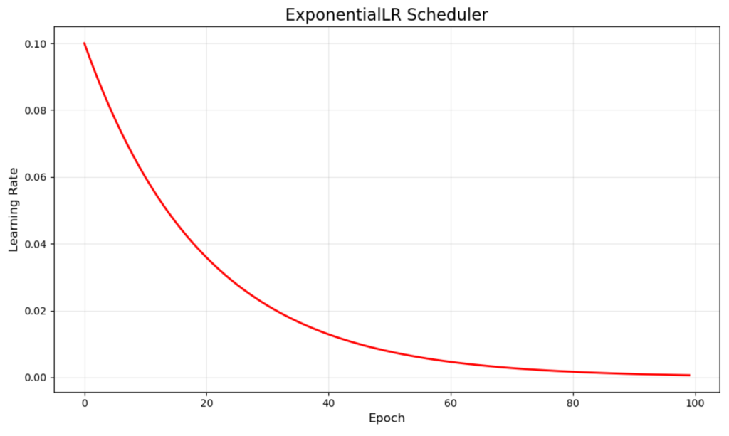
This continuous attenuation ensures that the model is always getting smaller and smaller as the training progresses. This can ruin training momentum, which is especially effective for problems where you want to improve step by step without a sharp transition.
The smoothing nature of exponential decay usually results in stable convergence, but the decay rate needs to be carefully adjusted to avoid reducing the learning rate too fast or too slow.
cosineannealinglr – cosine annealing
cosineannealinglr follows the cosine curve, starting from high to minimum. The green curve shows this elegant mathematical progress, which naturally slows down the change when it approaches the minimum.

This scheduler is inspired by simulated annealing and is widely popular in modern deep learning. The shape of the cosine provides more training time at a higher learning rate early on, and then gradually transitions to the fine-tuning phase.
Research shows that cosine annealing can help models escape local minimums and generally achieve final performance better than linear attenuation plans, especially in complex optimized landscapes.
ReDucelRonplateau – Adaptive Plateau Reduction
ReDucelRonplateau only takes a different approach when it improves stagnation and lowers learning rates. Purple visualization shows typical behavior around the declines in the 25, 50 and 75 periods.
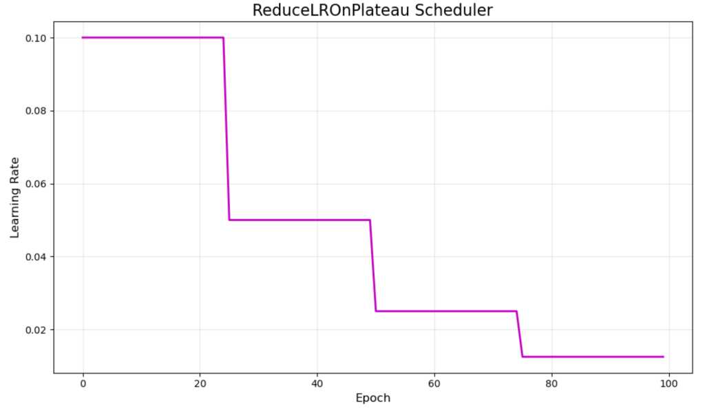
This adaptive scheduler responds to actual training progress rather than following a scheduled schedule. It reduces the learning rate when the verification loss stops improving the specified number of periods (Participation parameters).
The main advantage is its ability to react to training dynamics, which is very useful for situations where the best plan is uncertain. However, it requires monitoring of validation metrics and may respond slowly to the required adjustments.
Environmental protection – periodic learning rate
The cyclic layer oscillates in a triangle pattern with a minimum learning rate and a maximum learning rate. Our orange visualization shows these cycles, with rates climbing from 0.001 to 0.1 and downwardly downward during 40 school hours.

This approach pioneered by Leslie Smith challenges the traditional idea of only reducing learning rates. The theory suggests that periodic increase helps the model escape poorer local minimums and explores the loss surface more efficiently.
While periodic learning rates can achieve impressive results and are often trained faster than traditional methods, they require careful adjustment of the minimum, maximum and period length parameters to work effectively.
Actual implementation: MNIST example
Now, let’s take a look at the performance of these schedulers. We will train a simple neural network on the MNIST digital classification dataset to compare how different schedulers affect training performance.
Setup and data preparation
We first need to import the necessary libraries and prepare the data. The MNIST dataset contains handwritten numbers (0-9), which we will use a basic two-layer neural network for classification.
|
1 2 3 4 5 6 7 8 9 10 11 12 13 14 15 16 17 18 19 20 twenty one |
#Learning Rate Scheduler – Concise MNIST Demo import numpy As NP import Food potlib.PYPLOT As plt import Tensor As TF from Tensor.Difficult import layer,,,,, Callback from Tensor.Difficult.Optimizer import Adam import warn warn.Filter War((‘neglect’) #Data preparation ((x_train,,,,, y_train),,,,, ((x_test,,,,, y_test) = TF.Difficult.Dataset.mnist.load_data(() x_train,,,,, x_test = x_train / 255.0,,,,, x_test / 255.0 x_train = x_train.Reshape((–1,,,,, 784)[:10000] y_train = TF.Difficult.UTILS.to_categorical((y_train,,,,, 10)[:10000] #Simple Model defense create_model((): return TF.Difficult.order(([ layers.Dense(128, activation=‘relu’, input_shape=(784,)), layers.Dense(10, activation=‘softmax’) ]) |
Our model is intentionally simple – a hidden layer with 128 neurons. We used only 10,000 training samples to speed up the experiment while still demonstrating the scheduler’s behavior.
Scheduler implementation
Next, we implement each scheduler. Most schedulers can be used as a simple function to adopt the current era and learning rate and then return to the new learning rate. However, ReduceLROnPlateau Since verification metrics need to be monitored, the way they work is different, so we will deal with them separately in the training section.
|
1 2 3 4 5 6 7 8 9 10 11 12 13 14 15 16 17 18 19 20 twenty one twenty two twenty three twenty four |
#Learning rate schedule (match visualization parameters) defense step_lr((era,,,,, LR): #stepr: step_size = 20, gamma = 0.5 (from visualization) return LR * 0.5 if era % 20 == 0 and era > 0 Something else LR defense exp_lr((era,,,,, LR): #ExponentialLR: Gamma = 0.95 (from visualization) return LR * 0.95 defense cosine_lr((era,,,,, LR): #cosineannealinglr: lr_min = 0.001, lr_max = 0.1, max_epochs = 100 (from visualization) lr_min,,,,, lr_max = 0.001,,,,, 0.1 max_epochs = 100 return lr_min + 0.5 * ((lr_max – lr_min) * ((1 + NP.cos((Times * NP.pi / max_epochs)) defense Periodicity_lr((era,,,,, LR): #cyclicalallr: base_lr = 0.001, max_lr = 0.1, step_size = 20 (from visualization) base_lr = 0.001 max_lr = 0.1 STEP_SIZE = 20
cycle = NP.ground((1 + era / ((2 * STEP_SIZE)) x = NP.Abdominal muscles((era / STEP_SIZE – 2 * cycle + 1) return base_lr + ((max_lr – base_lr) * Maximum((0,,,,, ((1 – x)) |
Note how each feature implements the exact same behavior as shown in our earlier visualizations. Select the parameters carefully to match these patterns. ReduceLROnPlateau Special handling is required because it monitors verification losses during training and you will see us as callback settings in the next section.
Training and comparison
We then create a training feature that can use any of these schedulers and perform each scheduler: